01In short
Almost every tissue sample in a hospital gets stained pink and purple ("H&E") and photographed — it's cheap and routine. Measuring exactly which proteins are present, and where, takes a separate, much more expensive test called spatial proteomics.
My project asked: can a computer predict the expensive result from the cheap image? I treated each cell in the slide as a point in a network, connected it to its neighbours, and trained a graph neural network to predict the expression of 64 proteins in every cell.
I built this with Brennan Simon in the Curtis Lab and presented it in August 2025 as "Hematoxylin & Eosin (H&E) to Spatial Proteomics GNN." Everything below comes from that presentation.
02What I did
- Developed a graph convolutional network (GCN) that predicts spatial protein expression from H&E-stained whole-slide images.
- Combined three kinds of information about each cell: its predicted cell type, its position, and which cells it touches.
- Predicted the expression of all 64 CosMx proteins in every cell.
- For the 5 best-predicted proteins, achieved statistically significant agreement with the real measurements in 63% of evaluated comparisons, showing that molecular information can be inferred from ordinary histology.
03Two ways to look at tissue
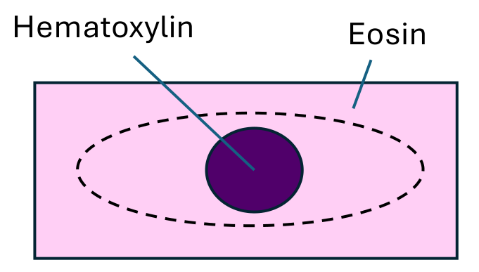
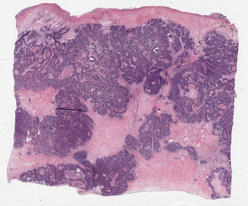
H&E staining is the clinical gold standard. It stains cell nuclei purple (hematoxylin) and the cytoplasm and surrounding tissue pink (eosin). It's cheap, fast, follows a standardized protocol, and is performed on every clinical biopsy. The catch is that it carries only low-level information.
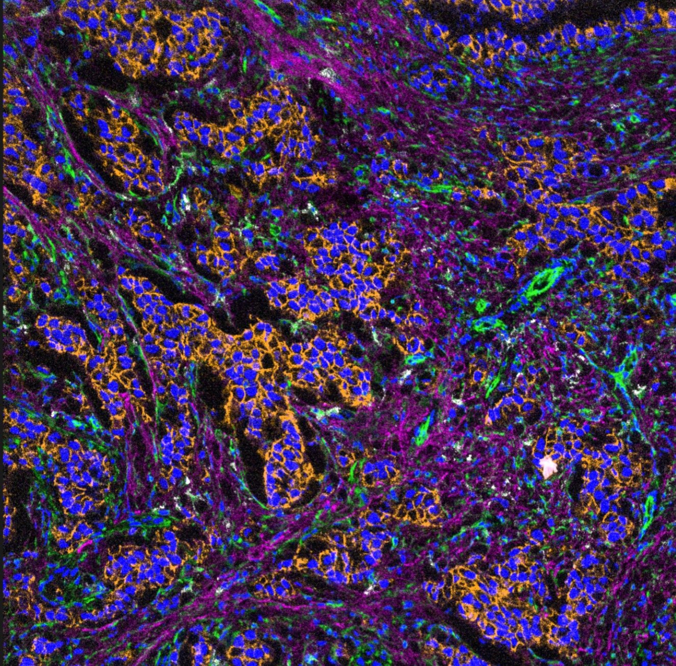
Spatial proteomics (here, the CosMx platform) measures dozens of proteins inside every single cell, at 40–64 targets at a time. It's extraordinarily detailed, but very expensive and slow. It covers a limited field of view and needs samples stored in particular ways.
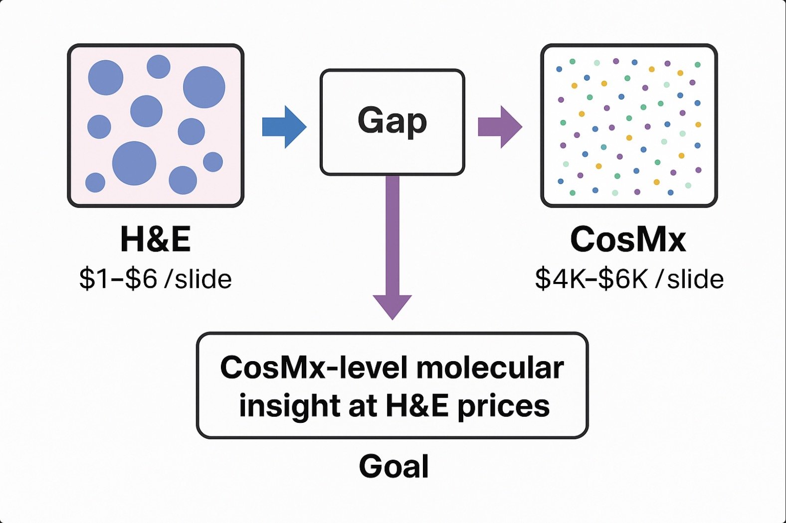
| H&E stain | 64-plex CosMx | 1000-plex CosMx | |
|---|---|---|---|
| Cost per slide | $1–6 | $3,880 | $5,996 |
04Why this project exists
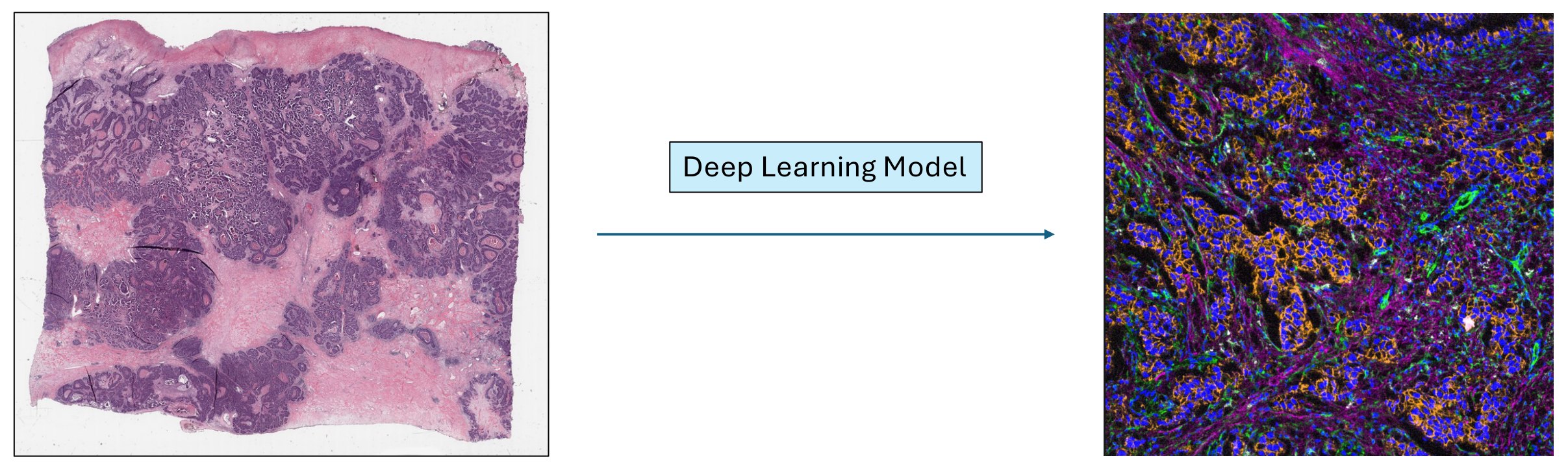
Close the gap between the two: CosMx-level molecular insight at H&E prices. A deep learning model takes the cheap H&E image in and predicts the expensive spatial proteomics picture out.
Clinical
Predict cell types and cell activity efficiently from data hospitals already collect, to help doctors make better diagnostic and treatment decisions.
Research
Impute complex spatial information from cheap, plentiful existing data, transforming what current spatial "omics studies can do and opening the door to new discoveries.
05The data
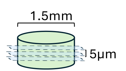
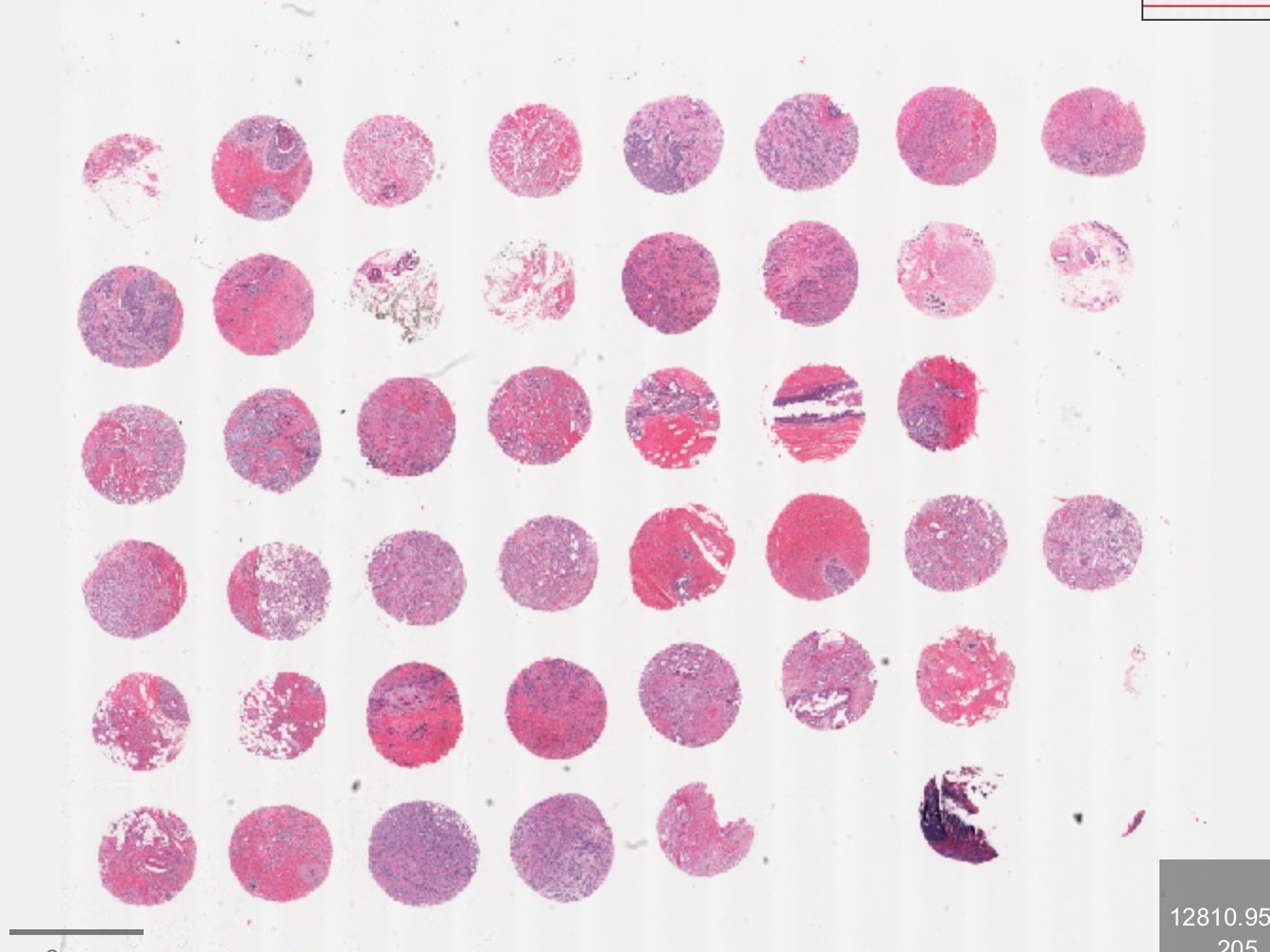
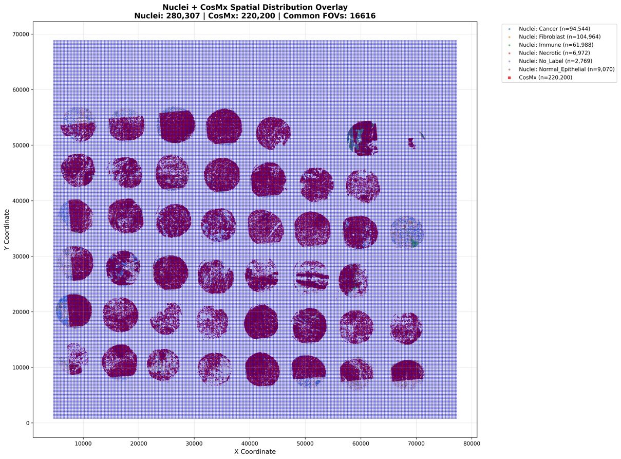
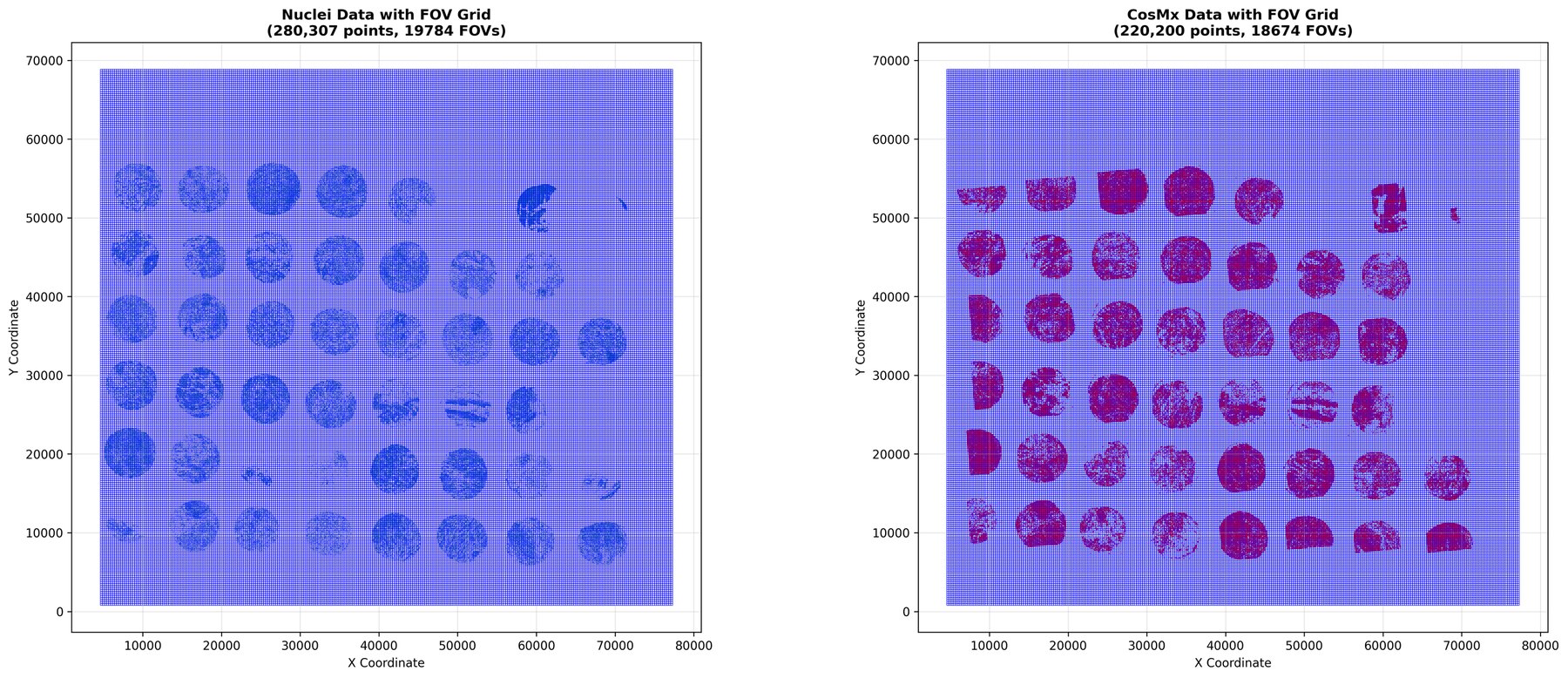
We used the Madrid cohort: six whole-slide images of tissue microarrays (TMAs), each with H&E and overlaid CosMx spatial proteomic data from the same tissue.
- 280,307nuclei detected in H&E
- 220,200cells measured by CosMx
- 16,616fields of view shared by both
Nuclei by cell type: fibroblast 104,964 · cancer 94,544 · immune 61,988 · normal epithelial 9,070 · necrotic 6,972 · unlabelled 2,769.
06From slide to graph
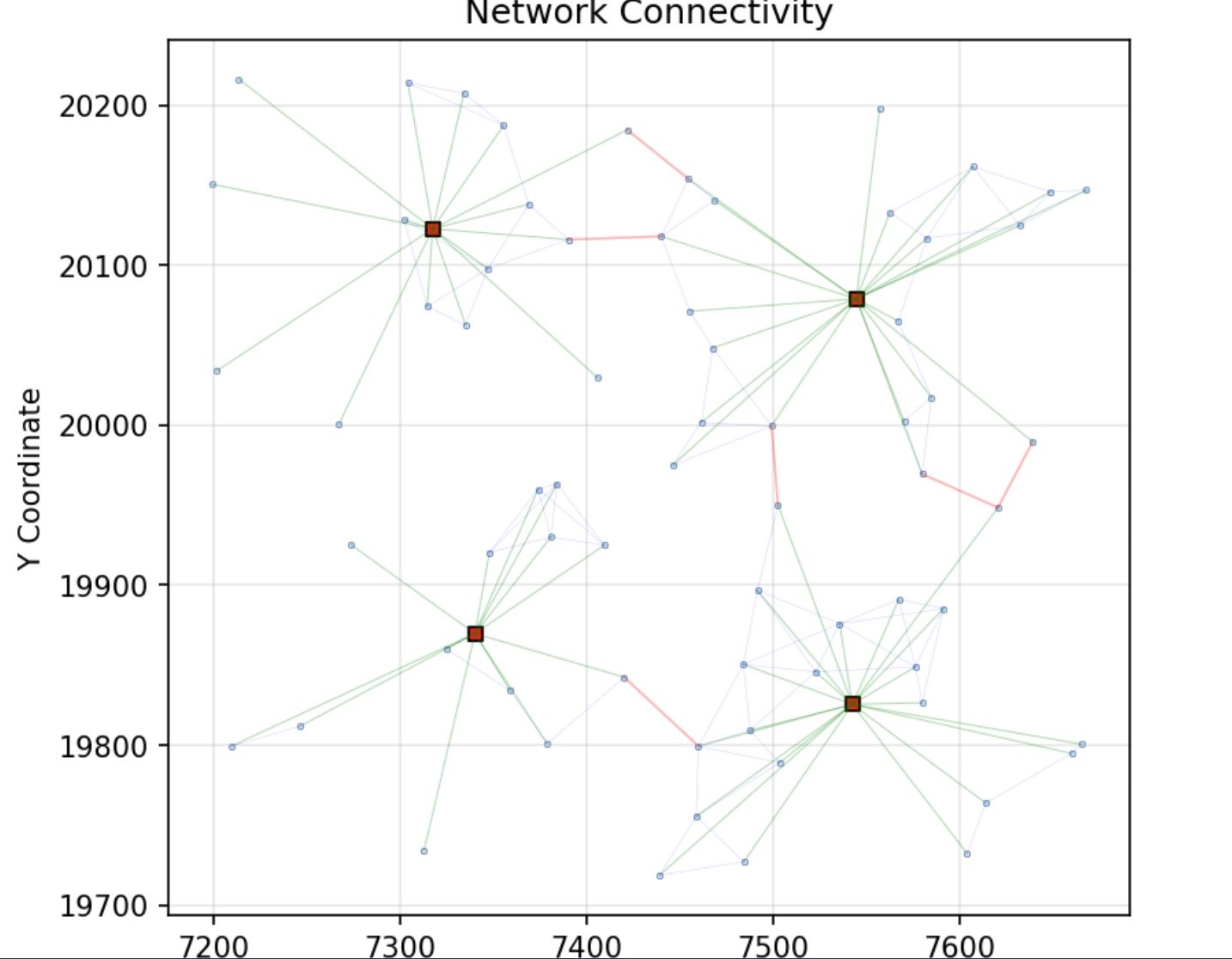
The core idea is to represent tissue as a graph. Each cell is a node, and edges connect cells that sit next to each other. The same graph is built twice over the same patch of tissue: once from H&E (the input) and once from spatial proteomics (the answer the model learns to predict).
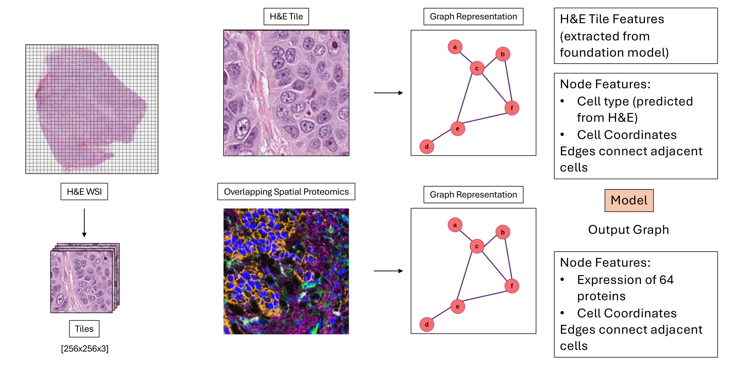
Building those graphs took a pipeline of several models:
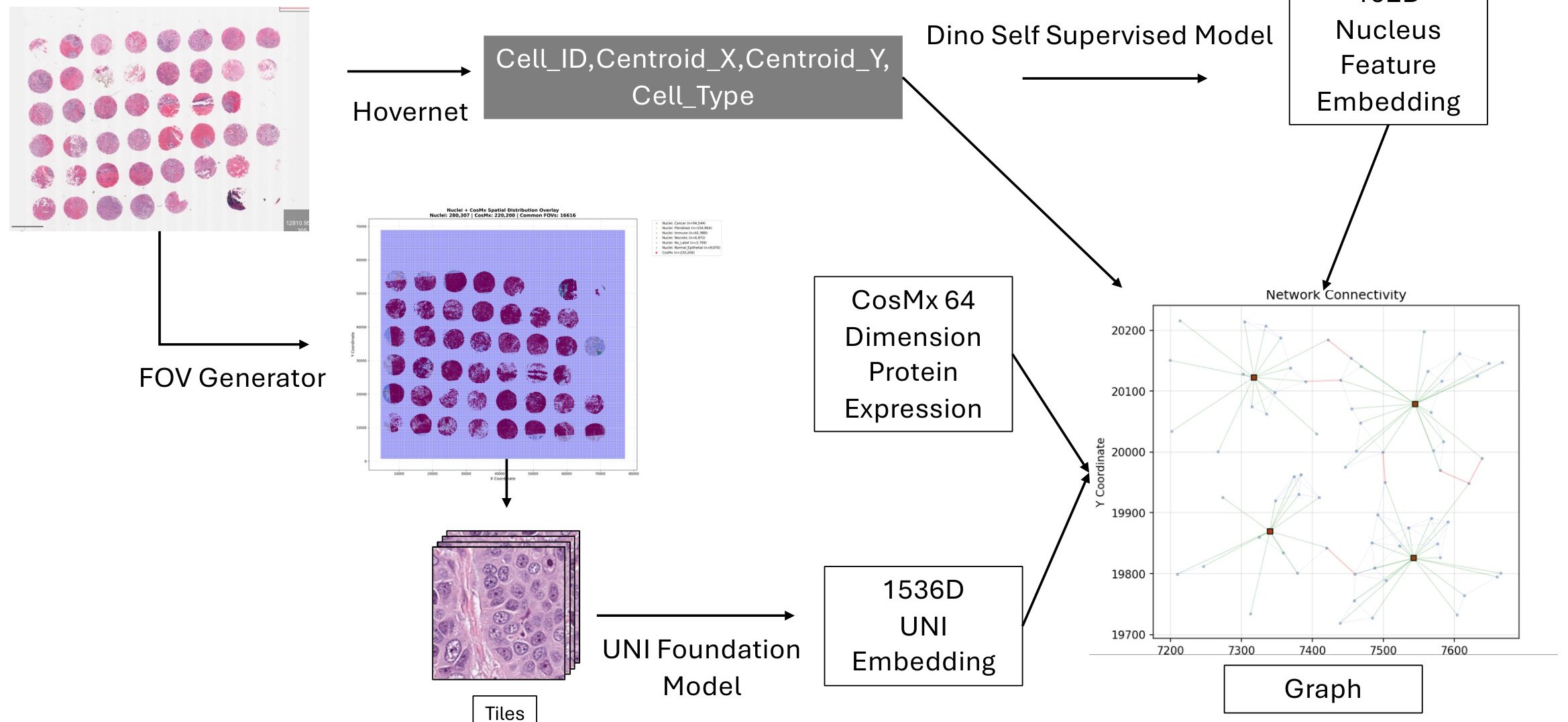
- HoverNet finds every nucleus in the H&E slide and outputs its ID, centroid (x, y), and cell type. It's a CNN built for nucleus segmentation and classification that accurately separates nuclei in dense tissue, labels each one (epithelial, lymphocyte, stromal, and so on), and is widely benchmarked on the PanNuke and CoNSeP datasets.
- DINO, a self-supervised model we trained ourselves, turns each nucleus into a 192-dimensional feature embedding.
- An FOV generator cuts the slide into 256×256-pixel tiles (fields of view).
- UNI, a self-supervised foundation model trained on millions of histology images, turns each tile into a 1,536-dimensional embedding that captures morphology, texture and tissue context, and generalizes across stains and tissue types.
- CosMx supplies the target: 64-dimensional protein expression for every cell.
07Generating fields of view
The FOV grid is calculated as 256×256-pixel squares from the top-left of each whole-slide image to the bottom-right. It serves three purposes: it's the unit for extracting UNI features, it's how per-FOV graphs are constructed, and it keeps spatial relationships manageable across a huge slide. It also puts a smaller load on the GPU when training the GNN.
08Teaching a model what nuclei look like
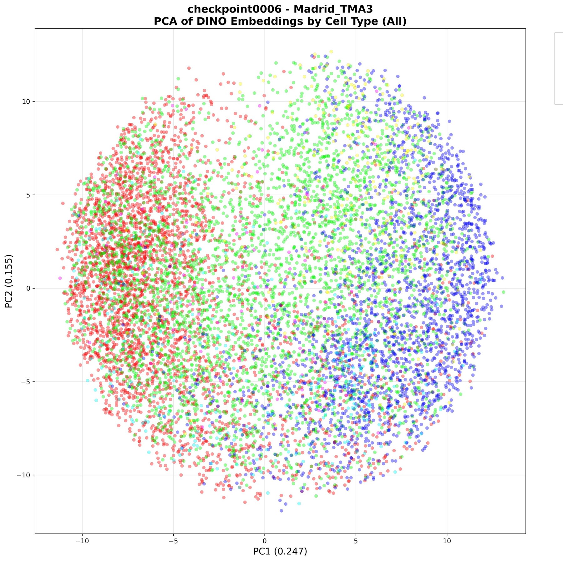
To describe each nucleus, we trained DINO, a self-supervised vision transformer from Facebook AI Research, on 1.7 million nuclei from the Madrid cohort. It produces a 192-dimensional embedding of each nucleus's features.
- A student and a teacher network, both vision transformers; the teacher is an exponential moving average (EMA) of the student.
- Multi-crop training: 2 global views (224 px) plus K local views (92 px) of each image.
- Loss: cross-entropy between the student's and teacher's outputs.
- Kept stable with the EMA update, centering, and temperature scaling.
- The result: view-invariant, transferable embeddings.

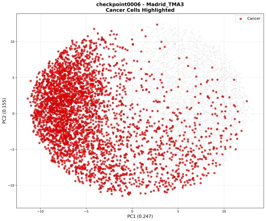
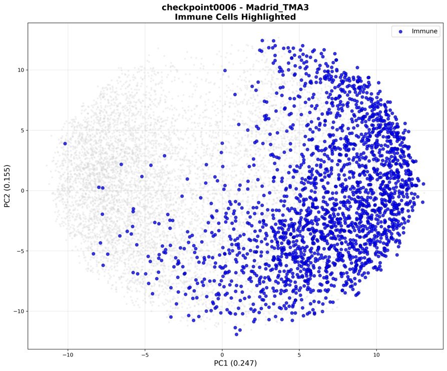
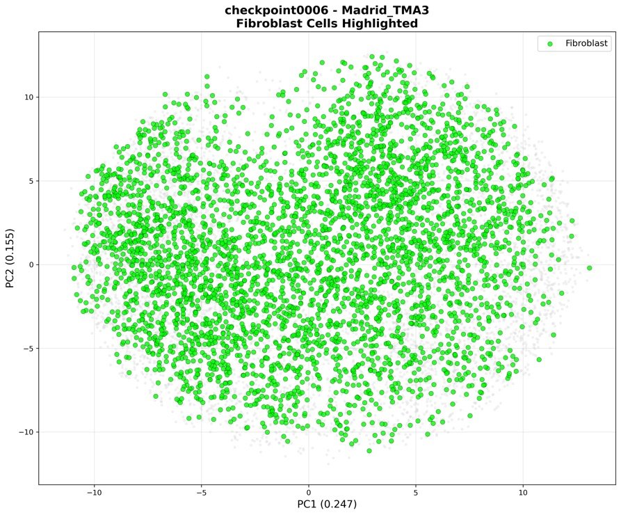
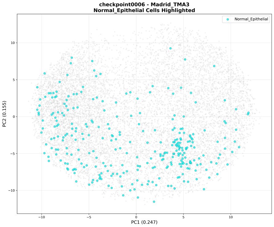
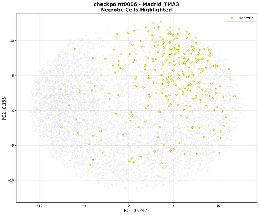
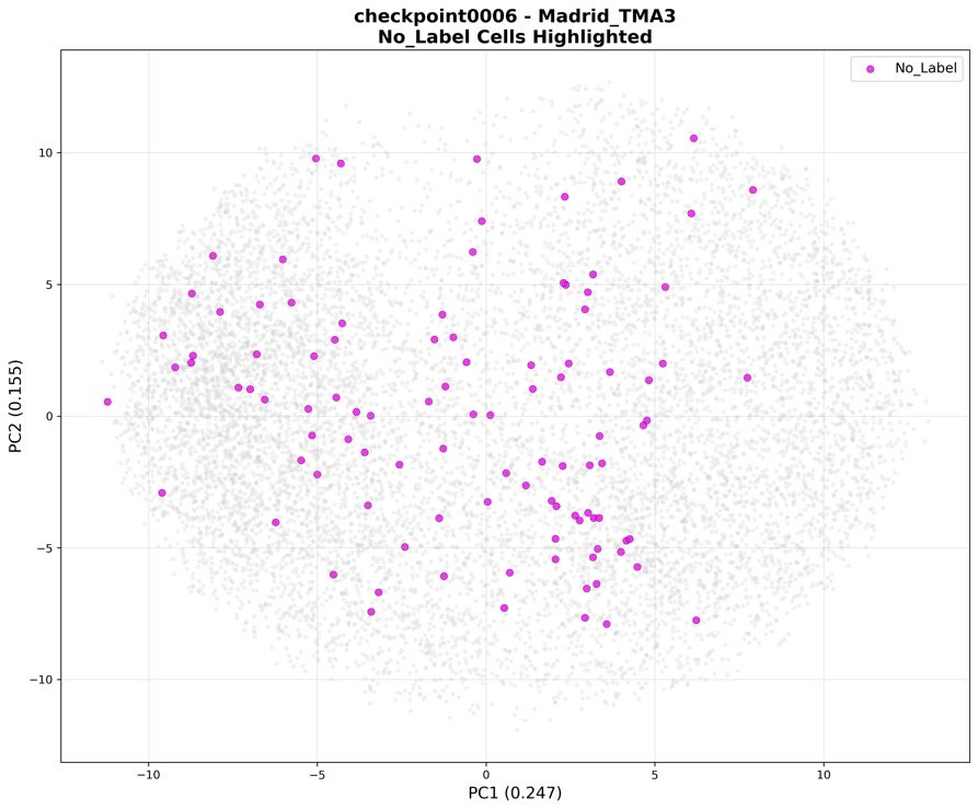
Without ever being told what cell types are, the trained model separates them. Plotting the embeddings (PCA), cancer, immune and fibroblast cells fall into distinct regions.
09Inside the graph
Inputs
- H&E nucleus features: morphology, cell type, x/y position.
- Spatial proteomics: 64 proteins per cell.
- UNI embeddings: a 1,536-dim representation of each FOV.
Sliding windows
- Groups 2×2 FOVs into one window, with a stride of 1.
- Each window must meet requirements: at least 20 cells, exactly 4 FOVs, and spatial proteomics mapping present.
Nodes
- Cell nodes: nuclei with H&E features, mapped to their proteins where available.
- Hypernodes: one per FOV carrying its UNI embedding, connected to all of that FOV's cells.
Edges
- Intra-FOV: connect neighbouring cells within 60 µm.
- Inter-FOV: connect cells across FOV boundaries.
- Hypernode edges: connect each UNI hypernode to its cells.
10The model
h′i = σ ( W · Σj ∈ 𝒩(i) hj / √(di dj) )
Each GCN layer updates a cell by averaging its neighbours' features, weighted by how connected each cell is (d = node degree).
- Cell-type embedding:
nn.Embedding(num_cell_types, 32) - Input projection:
Linear(input_dim + 32 → hidden_dim)+ ReLU + Dropout - GCN backbone:
num_layers × [GCNConv(H, H) → BatchNorm1d(H) → ReLU → Dropout] - Prediction head:
concat(final H, cell_type_emb) → MLP → 64 outputs - Loss: MSE · Optimizer: AdamW · LR scheduler: ReduceLROnPlateau
11Training
- 65,000graphs for training
- 10,000held out for validation
- 6 hrsper epoch
- 2epochs in total
12Results, for now
After two epochs, the results split in two.
Five proteins came through. For the 5 best-predicted proteins, the model's predictions agreed with the measured CosMx expression with statistical significance in 63% of evaluated comparisons. That's the core evidence that molecular information can be read from ordinary H&E histology.
Most of the other proteins are still poorly predicted. Across the full panel of 64, the correlation between predicted and measured expression mostly sits between about 0.05 and 0.2, and 15 proteins came out negative.
That's a starting point rather than a failure. The pipeline works end to end, the DINO embeddings clearly capture biology, five proteins already show real signal, and the results show exactly where to push next.
13Next steps
- Retraining with a higher batch size.
- Extended training: more epochs, plus hyperparameter sweeps over learning rate, dropout and loss functions.
- Feature extraction: replace or augment DINO with a chopped HoverNet, to get more H&E nuclei for training.
- Graph construction: try different edge definitions: k-nearest neighbours, radius, and distance-weighted edges.